Roughly 20 years ago, I built a 7 element Yagi-Uda antenna after a design by DK7ZB. The antenna was stored somewhere in the garage for the last 15 years and needs some polishing before I can get on the air again. As measurement technology evolved quite a bit since then, a lot can be learned along the way. I plan to do a small series of articles about that.

Estimating the Velocity Factor of an Unknown 75Ohm Cable

As the antenna is a 28Ohm design, a quarter-wave transformer from two 75Ohm cables is needed to match the antenna to the standard 50Ohm. As I have a significant amount of 75Ohm cable from my house’s installation lying around, I decided to use that. However, although there is a datasheet available, this datasheet is more a brochure and does not list the velocity factor of the cable. The basic process to do this is straight forward: Measure the mechanical length, measure the electrical length and divide one through the other.

Measuring the Electrical Length of a Coaxial Cable (The Simple but Wrong Solution)

The electrical length of can be easily measured by \(l_e=\lambda \frac{\varphi}{2\pi}\). With this, the following graphs can be obtained for an \(s_{11}\) measurement of a 2.75m long piece of cable with an open end.

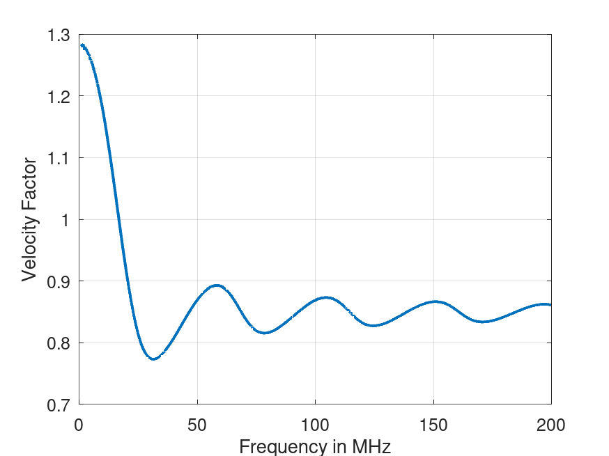
So obviously this does not work (for most frequencies). The explanation is quite simple: The NanoVNA and my calibration kit are 50Ohm, the cable is 75Ohm. This is why reflections occur at the transition between the different impedance domains and not only at the open end of the cable under test. This results in a superposition of multiple waves which spoil the phase measurement.

Measuring the Electrical Length of a Coaxial Cable (The Complicated Solution)

In order to understand the different signals on the lines, a model can be formulated:

\(s_{11} = \Gamma + (1+\Gamma)(1-\Gamma) \sum^i_{1…n}(-\Gamma)^{i-1}e^{2\pi\text{j}\frac{i2l_e}{\lambda}}\),

with the reflection factor from the transition from 50Ohm to 75Ohm \(\Gamma = \frac{75-50}{75+50}=0.2\). The terms \(1+\Gamma\) and \(1-\Gamma\) are the transmission coefficients to the 75Ohm domain and back to 50Ohm. It can be larger than 1 because we are considering voltages. The term \(-\Gamma\) results from the reflection at the transition from 75Ohm to 50Ohm \(\frac{50-75}{50+75}=-0.2=-\Gamma\). The exponential term represents the different signals with the actual length they traveled proportional to the number of round trips. Finally, the following graphs can be obtained:

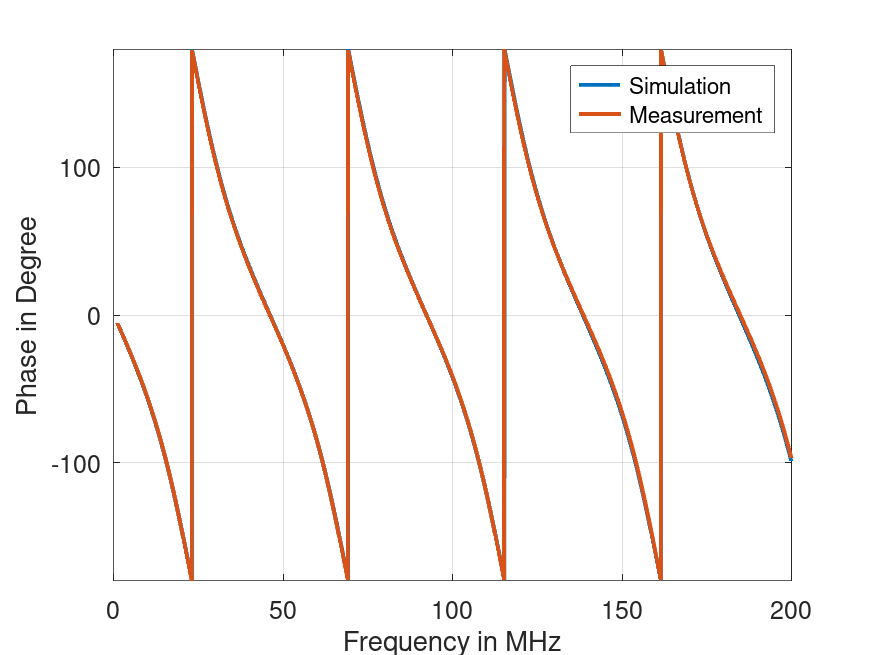
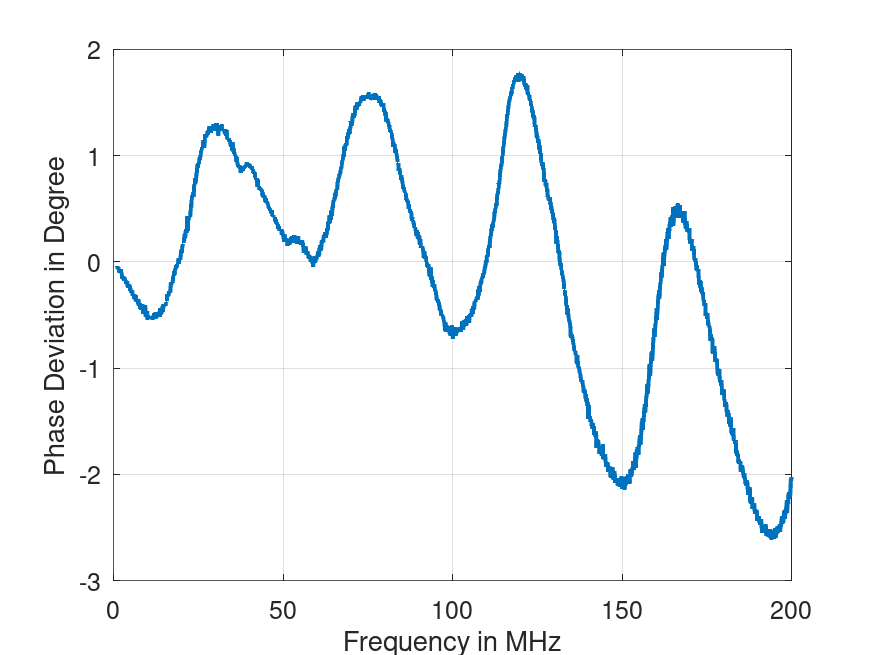
On the left side, the measurement overlays the simulation which is a good sign. In the end, the parameters for the equations leading to the graphs shown above have been found by very complex mathemagical optimization trial end error, resulting in an estimation of \(v_f \approx 0.85\). There is still a deviation between the measured and the modeled phase but as I did not model the loss of the cables, the accuracy of a few degrees is good enough for my standards.

Measuring the Electrical Length of a Coaxial Cable (The Simple Solution)

When looking at the model equation above, one can see that all contributions are periodic with the electrical length and multiples of it. This means, when looking at the plot of the unwrapped phase, one can simple look for two points with the same phase, take the difference of the allocated frequencies and take the electrical length as the wavelength of that frequency. This can be done using a Fourier transform (FT) of \(s_{11}\) and finding the first peak or just graphically by hand. As for the FT-based approach, the measurement bandwidth of 200MHz results in a low range resolution, zero padding was applied to get a better estimate. From this graph one can also see that at least 5, maybe 6 round trips can be resolved using the chosen parameters of my measurement setup before the noise and maybe other effects takes over.

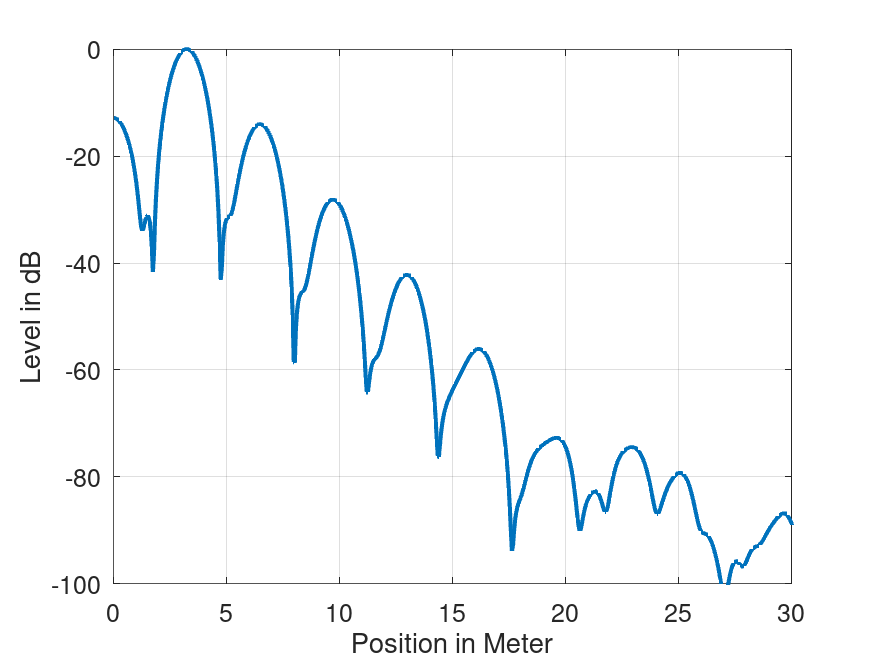
When zooming in a bit, one can find the electrical length from the FT plot to be 3.23m (the first peak). Together with the mechanical length of 2.75m this leads to the same velocity factor as above: \(v_f \approx 0.85\). When read from the phase plot in the previous section, I get a frequency difference between the first two values closest to 180° of 46.2 MHz, which results in a half-wavelength of 3.24m what in the end also results in \(v_f \approx 0.85\).

Summary and Outlook

Within this short article, I presented different methods to evaluate the velocity factor of a cable with an impedance different from the measurement system. Although the result is consistent for the different methods, one should always keep in mind that the value obtained could also be found when looking up cables with foam dielectric (something between 80 and 90%). This accuracy is probably good enough for most practical purposes. However, with the analyses performed at least I learned something.

Finally, with the cable’s now known velocity factor, I can start building the quarter-wave transformer. As this is a complex topic, I will cover this in a separate article.