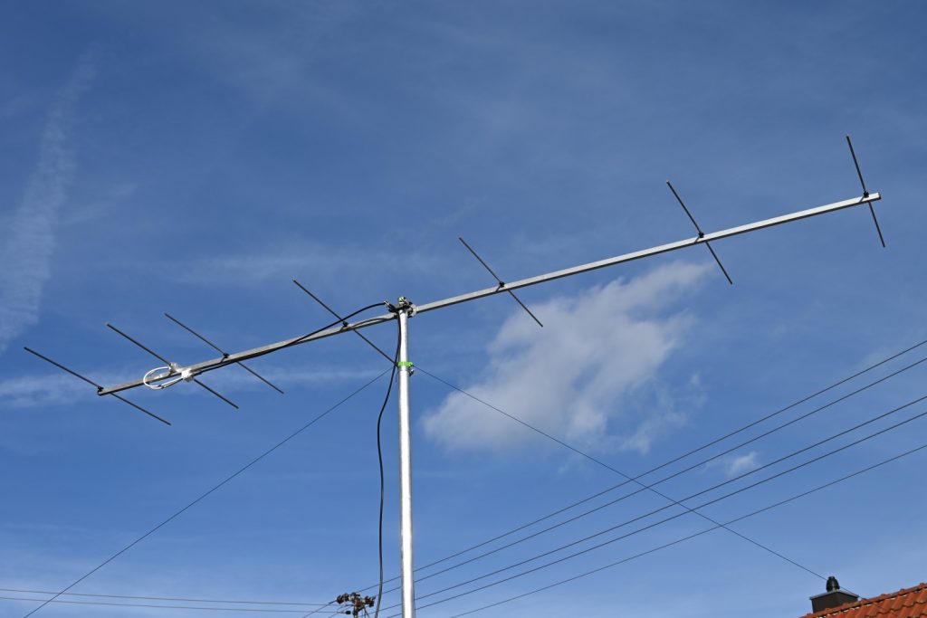
This is how the antenna looked after first assembly. It is not yet finalized in terms of feed line fixture and also the quarter wave transformation line needs some more care, but in general the setup works in sunny weather.
Tuning the Radiator
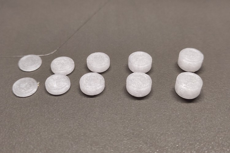
As it is typically very difficult to hit the correct length at first try, the usual approach is to leave the radiator a bit too long and cut it as required. As I ended up with a radiator that is too short at the beginning, I tried to lengthen it by inserting additional spacers in the center.
The printed spacers (1mm to 5mm)Dipole center with 5mm spacers
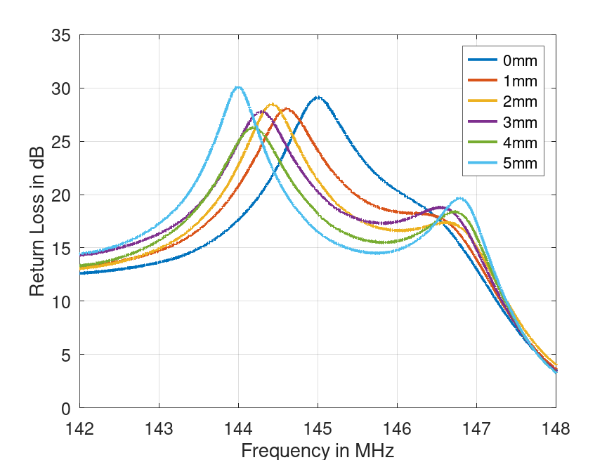
This actually helped and I could make a series of measurements to select the appropriate length. The return loss measurements are very good as expected. The results were obtained with calibration including the feed line to the antenna. As I do not have an N-type calibration kit, some imperfections due to the adapters I used remain which means the phase of the measurement is off by some degrees. Nevertheless, for amateur standards, the results should be acceptable.
Return loss over frequency for different spacer sizes.
The following table summarizes the results. As the spacing is applied on both sides of the dipole, the actual length is increased by twice the value. In the end, I ended up at the design frequency using the 3mm spacers. However, with the 1mm spacers, I would achieve the best performance over the whole 2m band.
Spacing / mm
0
1
2
3
4
5
Frequency / MHz
145.01
144.6
144.43
144.31
144.16
144.01
Maximum Return Loss / dB
29.1
28.1
28.5
27.8
26.3
30.1
Maximum return loss @ frequency for the different spacer sizes.
Performance Evaluation On the Air
I made some QSOs during the 2024 BBT contest in February with a not yet finished version of the antenna and also tried FT8 and the results looked promising. I could at least hear stations nearly 500km away although I had around 3dB loss in my feed line. However, with my old IC706Mk2G, the frequency stability on 2m is very challenging for the digital modes. It works with strong signals but real weak signal operation will need some improvement on this side.
Closing Remarks
With this article, the short series could be finished. However, there are some theoretical aspects I observed and I would like to elaborate in more detail. Therefore there might be a fourth article that covers these but this may take some time…
As I have never been operational on the 6m band, the plan to build a dedicated antenna for that band came up. Due to my space restrictions, I chose this design by DK7ZB because, as he writes, “all you need is gain”.
Mechanical Construction
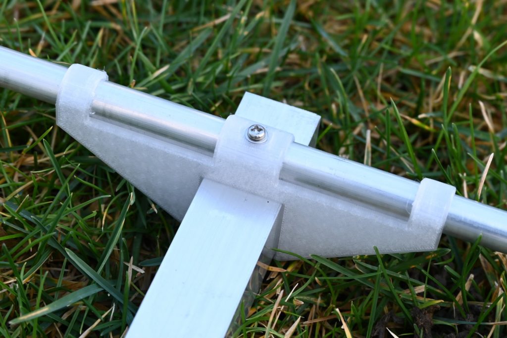
I used 25mm square aluminum tube as boom and all the elements are made from round aluminum tubes with 12mm diameter. As I did not find the right gear for that dimensions from the shops I typically use, everything was newly designed and 3D-printed as already shown in another article on the 144MHz Yagi-Uda antenna. The element holders were designed to go around the boom in order to offer some stability even without any screws. The screw through the element then adds the last bit of stability to keep the elements in place. Finally, the mast fixture was assembled from some parts from the local hardware shop.
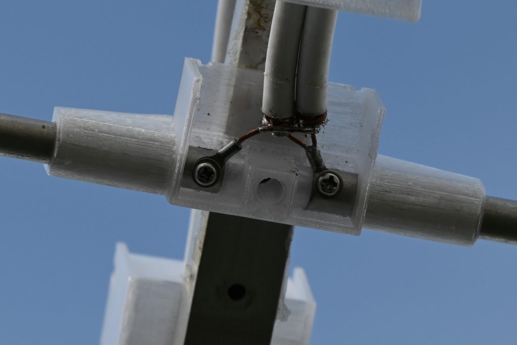
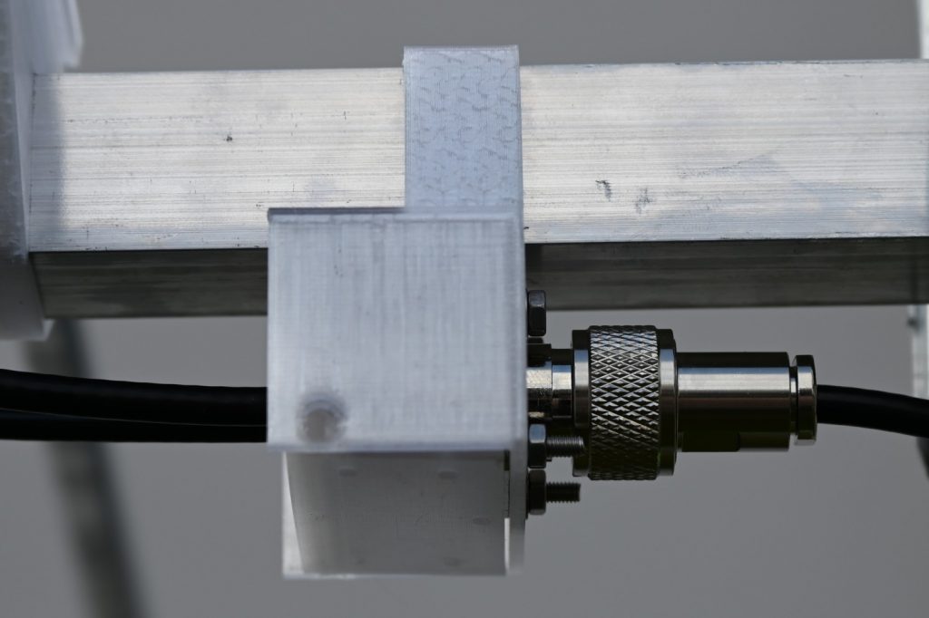
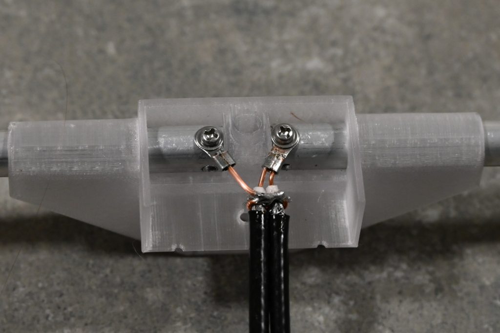
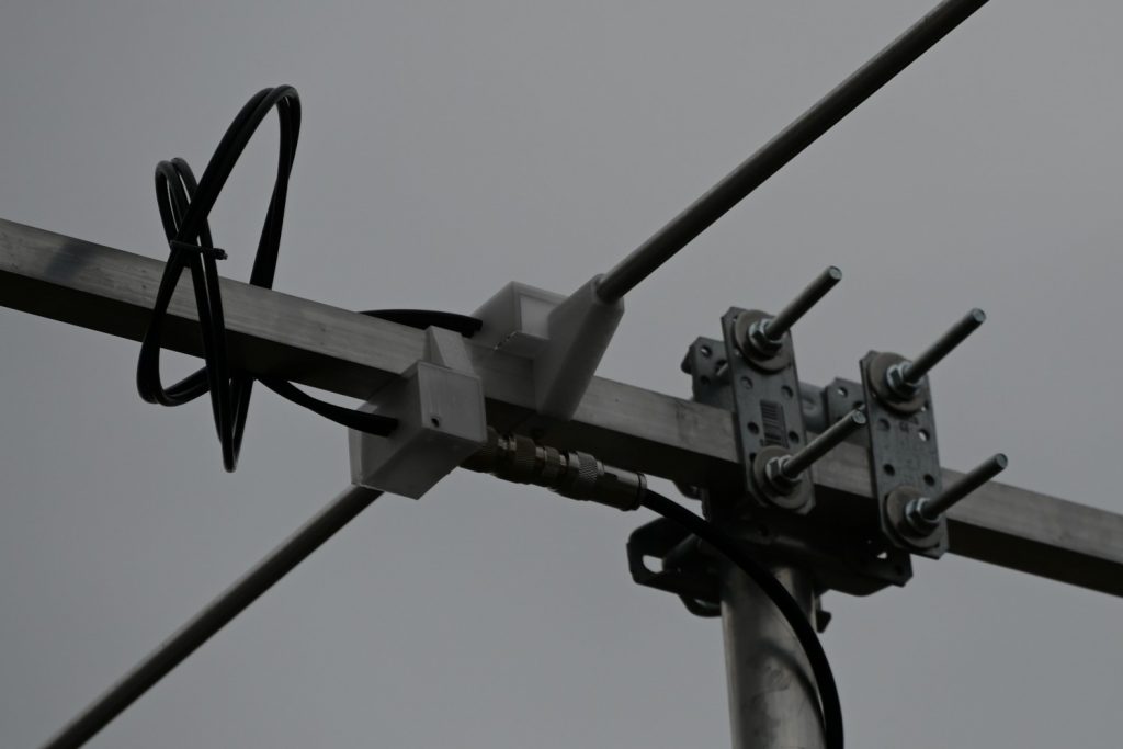
Element mountConnector boxDipole box with connectionDipole, connector and mast fixture
Electrical Construction
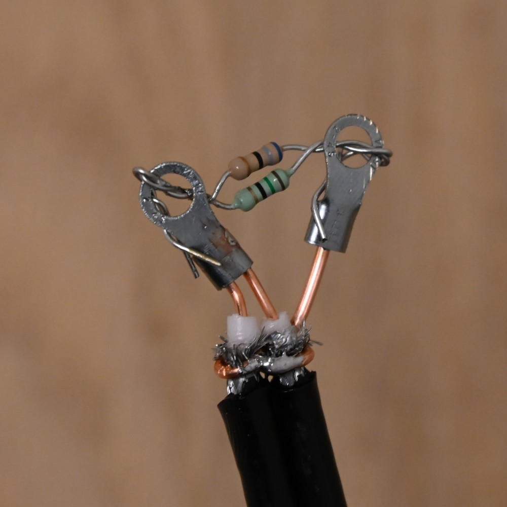
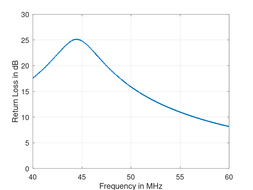
The antenna itself was designed with a feed impedance of 12.5Ohm and can be matched to 50Ohm using a quarter wave transformer with 25Ohm. This can easily be built with two parallel 50Ohm cables. The procedure itself is straight forward: Put a connector on one end of the two 50Ohm lines, a resistor with 12.5Ohm at the other end and adjust the length of the lines until you reached the lowest return loss at the desired frequency which is around 50MHz in this case. As for my other projects, the actual length required for the lines is way below the expected length using the wavelength and velocity factor. In the graph below, the return loss of the matching section is shown with the length about right according to frequency and velocity factor. Unfortunately, I forgot to save the final match at 50MHz.
Putting it all Together
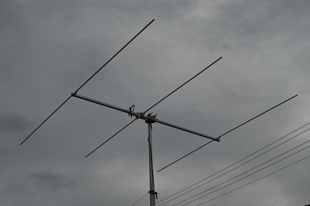
After putting the mechanics together with the matching network and mounting it on a mast, the optical result looks quite impressive in my small yard.
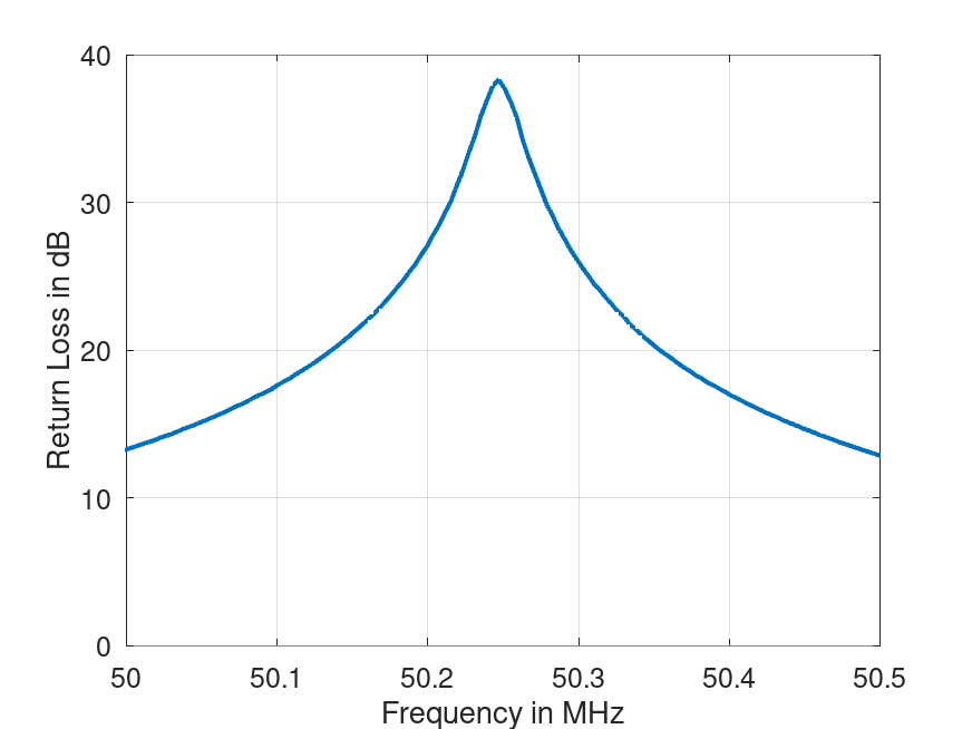
The resulting return loss is as expected very narrow and at a higher frequency as in the original design. This was expected to some degree because I used 12mm elements without 16mm inner parts as described by DK7ZB. According to EZNEC I should have ended at 50.28MHz which would be good for digital modes and SSB operation. As can be seen from the graph below, the maximum return loss of 38dB sits at 50.25MHz. From the graph one can read the 20dB bandwidth as 210kHz (from 50.14MHz to 50.35MHz) and the 13dB bandwidth to be 490kHz (from 50.0MHz to 50.49MHz) which is quite perfect for me.
Return loss of the final antenna with the measurement plane calibrated to the antenna’s feed point.
After some first trials, the results look promising but I am looking forward to real operation with this antenna while the conditions improve towards the summer.
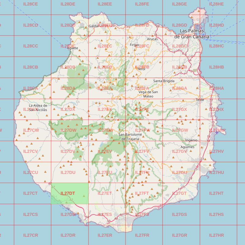
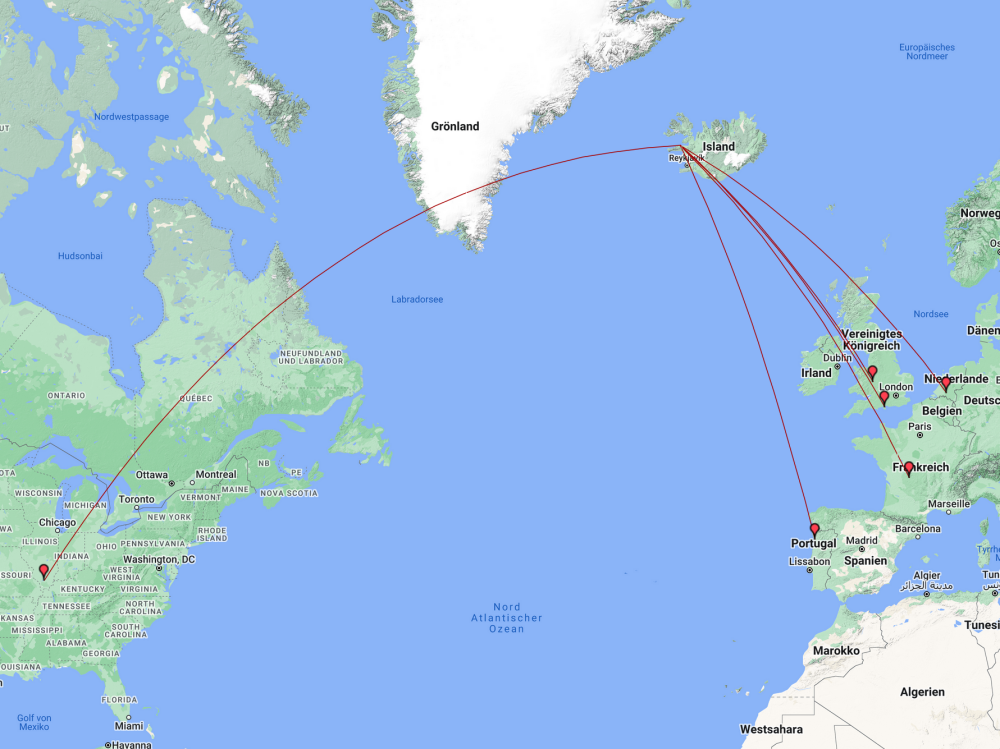
Last year in October, I have been active from a QTH in Gran Canaria with the same portable setup as I used in Iceland. The position on the island (locator IL27DT) and the QSO partners are shown in the two images below.
The following table summarizes the results. I am quite surprised how good this little setup performs. As can be seen from the number of QSOs, I ended operating mostly on the 10m band due to the good conditions.
There are a lot of builds online with different sources for material. Unfortunately, a lot of the referenced shops are already offline or do not sell the specific item anymore. This is where 3D-printing can help a lot…
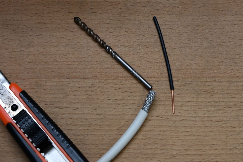
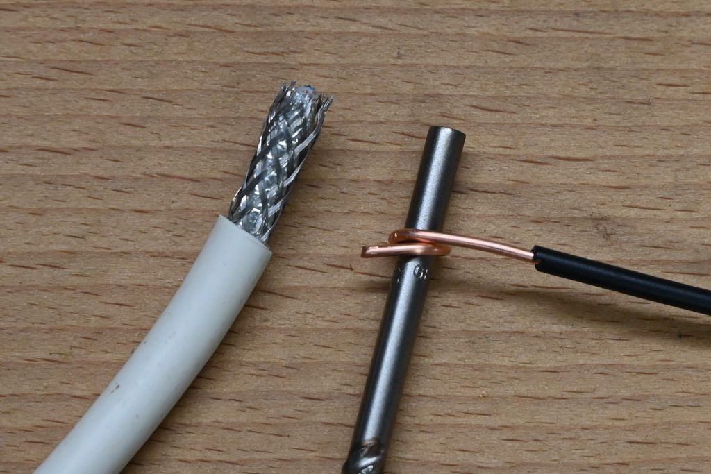
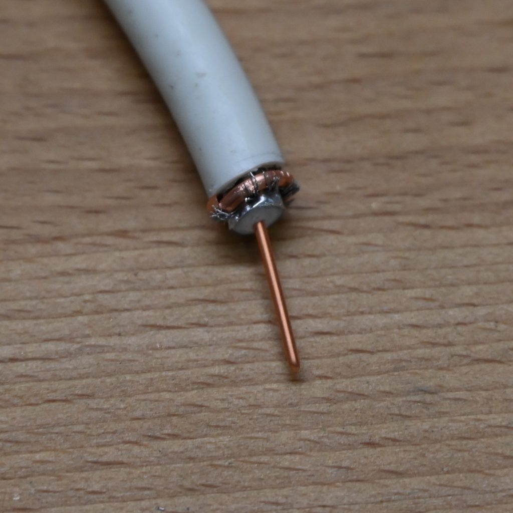
The Coaxial Cable
As the coaxial cable shielding is often made from aluminum, soldering is typically impossible. Therefore I used some 1.5mm² installation cable with solid core to produce smaller copper rings that in the end can be soldered. The process is illustrated in the pictures below.
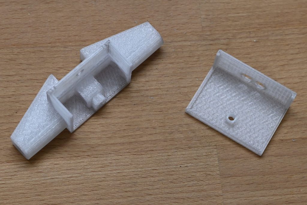
The Dipole Mount
For the dipole, I designed a mount that is as small as possible. I expect that the resonance frequency is reduced a bit by the length of the aluminum tube covered in PETG. In the pictures below, I mounted the old dipole as an exercise for drilling. To minimize the material and space requirements, I cut an M3 thread directly into the dipole tube. Time will tell if that is stable enough.
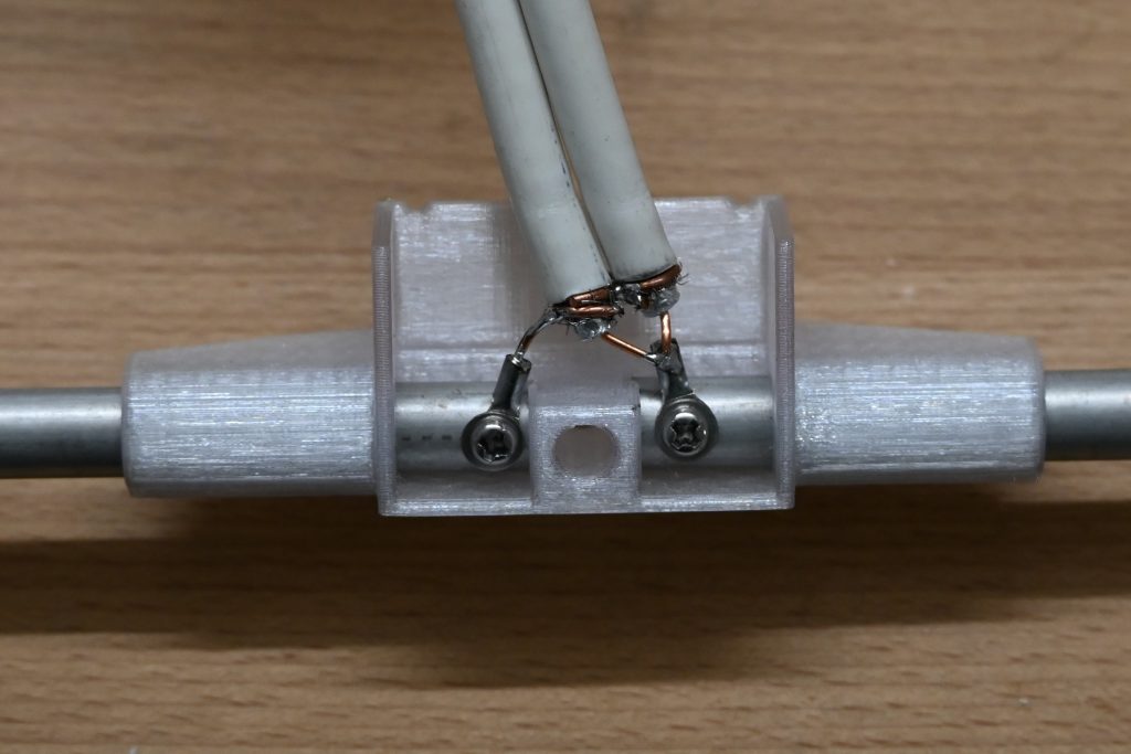
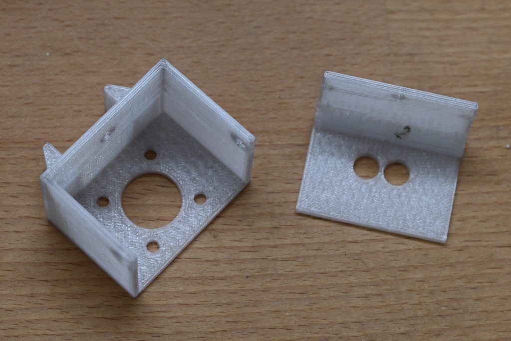
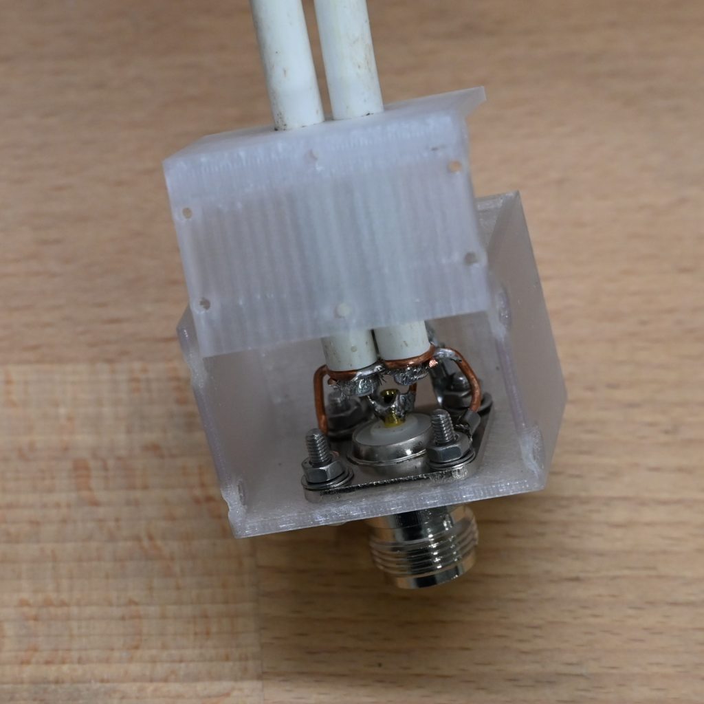
The Plug
The N-type plug will be mounted below the boom and also has it’s own custom designed housing. In the right picture, I tried to build the connection as symmetrical as possible with the copper rings as shown above.
The Element Mounts
Nothing to see here. Currently I just use the mounts available at the typical stores. In the future, I will be testing element holders very similar to my 3D-printed dipole holder. As this will have an influence on the elements’ electrical length, some investigation will be necessary.
Roughly 20 years ago, I built a 7 element Yagi-Uda antenna after a design by DK7ZB. The antenna was stored somewhere in the garage for the last 15 years and needs some polishing before I can get on the air again. As measurement technology evolved quite a bit since then, a lot can be learned along the way. I plan to do a small series of articles about that.
Estimating the Velocity Factor of an Unknown 75Ohm Cable
As the antenna is a 28Ohm design, a quarter-wave transformer from two 75Ohm cables is needed to match the antenna to the standard 50Ohm. As I have a significant amount of 75Ohm cable from my house’s installation lying around, I decided to use that. However, although there is a datasheet available, this datasheet is more a brochure and does not list the velocity factor of the cable. The basic process to do this is straight forward: Measure the mechanical length, measure the electrical length and divide one through the other.
Measuring the Electrical Length of a Coaxial Cable (The Simple but Wrong Solution)
The electrical length of can be easily measured by \(l_e=\lambda \frac{\varphi}{2\pi}\). With this, the following graphs can be obtained for an \(s_{11}\) measurement of a 2.75m long piece of cable with an open end.
So obviously this does not work (for most frequencies). The explanation is quite simple: The NanoVNA and my calibration kit are 50Ohm, the cable is 75Ohm. This is why reflections occur at the transition between the different impedance domains and not only at the open end of the cable under test. This results in a superposition of multiple waves which spoil the phase measurement.
Measuring the Electrical Length of a Coaxial Cable (The Complicated Solution)
In order to understand the different signals on the lines, a model can be formulated:
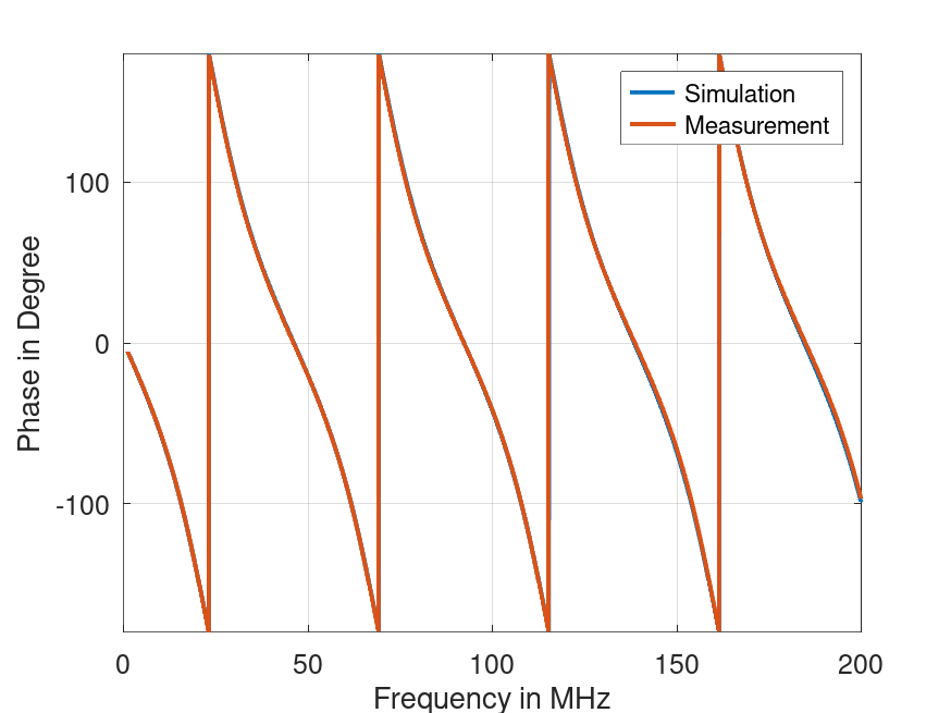
with the reflection factor from the transition from 50Ohm to 75Ohm \(\Gamma = \frac{75-50}{75+50}=0.2\). The terms \(1+\Gamma\) and \(1-\Gamma\) are the transmission coefficients to the 75Ohm domain and back to 50Ohm. It can be larger than 1 because we are considering voltages. The term \(-\Gamma\) results from the reflection at the transition from 75Ohm to 50Ohm \(\frac{50-75}{50+75}=-0.2=-\Gamma\). The exponential term represents the different signals with the actual length they traveled proportional to the number of round trips. Finally, the following graphs can be obtained:
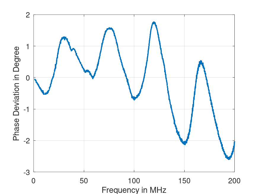
On the left side, the measurement overlays the simulation which is a good sign. In the end, the parameters for the equations leading to the graphs shown above have been found by very complex mathemagical optimization trial end error, resulting in an estimation of \(v_f \approx 0.85\). There is still a deviation between the measured and the modeled phase but as I did not model the loss of the cables, the accuracy of a few degrees is good enough for my standards.
Measuring the Electrical Length of a Coaxial Cable (The Simple Solution)
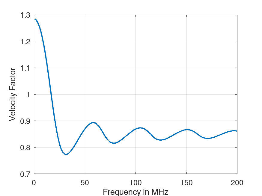
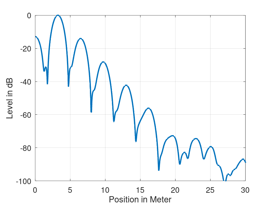
When looking at the model equation above, one can see that all contributions are periodic with the electrical length and multiples of it. This means, when looking at the plot of the unwrapped phase, one can simple look for two points with the same phase, take the difference of the allocated frequencies and take the electrical length as the wavelength of that frequency. This can be done using a Fourier transform (FT) of \(s_{11}\) and finding the first peak or just graphically by hand. As for the FT-based approach, the measurement bandwidth of 200MHz results in a low range resolution, zero padding was applied to get a better estimate. From this graph one can also see that at least 5, maybe 6 round trips can be resolved using the chosen parameters of my measurement setup before the noise and maybe other effects takes over.
When zooming in a bit, one can find the electrical length from the FT plot to be 3.23m (the first peak). Together with the mechanical length of 2.75m this leads to the same velocity factor as above: \(v_f \approx 0.85\). When read from the phase plot in the previous section, I get a frequency difference between the first two values closest to 180° of 46.2 MHz, which results in a half-wavelength of 3.24m what in the end also results in \(v_f \approx 0.85\).
Summary and Outlook
Within this short article, I presented different methods to evaluate the velocity factor of a cable with an impedance different from the measurement system. Although the result is consistent for the different methods, one should always keep in mind that the value obtained could also be found when looking up cables with foam dielectric (something between 80 and 90%). This accuracy is probably good enough for most practical purposes. However, with the analyses performed at least I learned something.
Finally, with the cable’s now known velocity factor, I can start building the quarter-wave transformer. As this is a complex topic, I will cover this in a separate article.
When booking a trip to Iceland, the idea emerged to become QRV on some HF bands in digital modes using my (tr)uSDX. As I did not want to take excessive luggage with me, the precondition was that the additional equipment has to be as small as possible. After some investigation and experiments, the following setup was used.
Hardware Setup
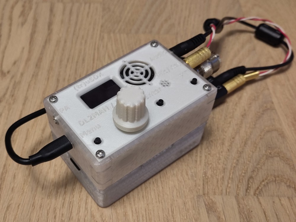
The TRX was of course decided beforehand to be the (tr)uSDX with the high band option (20m and up) for the antenna not to be too large. It is powered by a powerbank capable of providing 12V via USB PD and the necessary trigger device.
(tr)uSDX with 3D-printed housing combined with the Raspberry Pi and cabling.
The computer was also a simple decision: A Raspberry Pi 4 with 4GB of RAM with a small 3d-printed housing. It is powered from a different power bank directly with 5V via USB-C.
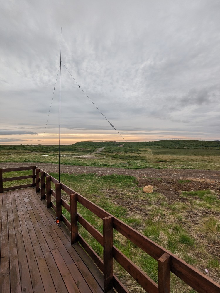
The hardest decision was the antenna, as antennas on the HF bands are typically large. In the end however, the decision was the obvious choice to use a linked end-fed antenna. It can be tuned by opening the respective connections. The center of the antenna is elevated with a telescopic fishing rod to about 4m height. Longer rods would of course be better but have a packed length that goes beyond the size of my suitcase. The connection between the TRX and the antenna is made using roughly 5m of Airborne 5 cable.
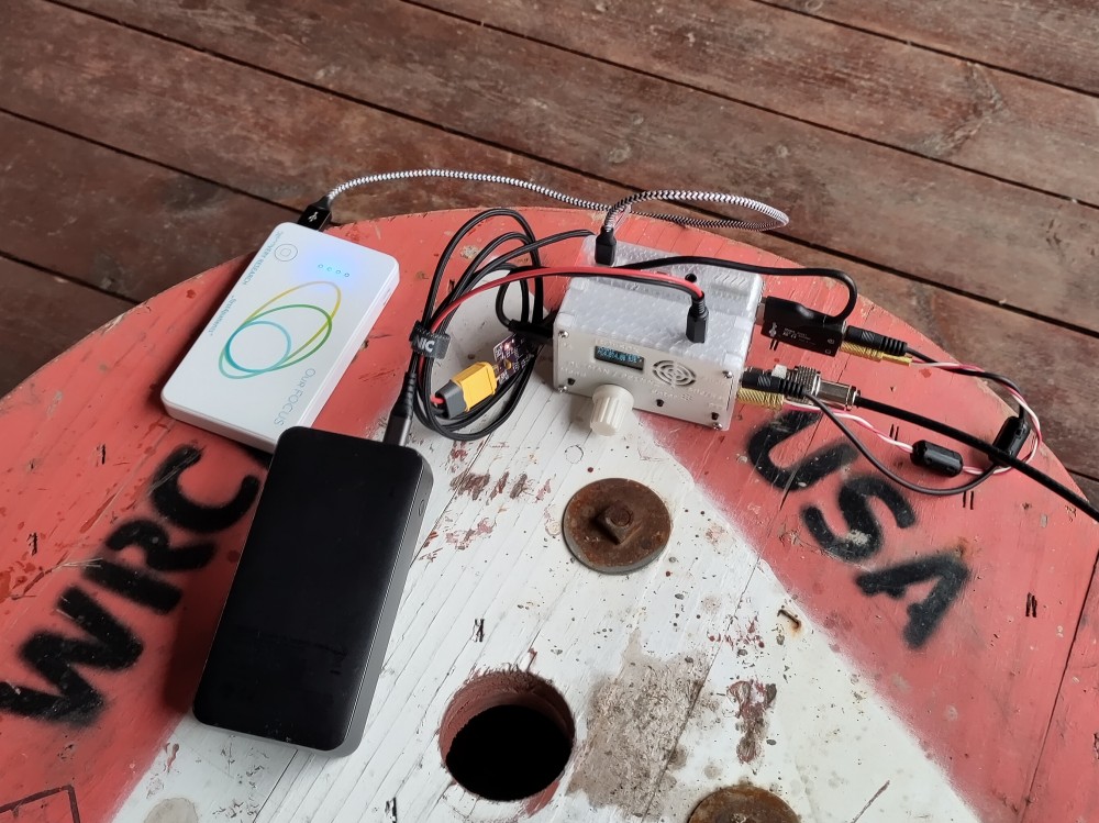
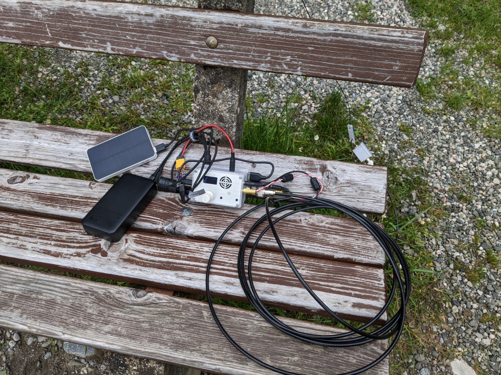
The full setup with powerbanks, Raspberry Pi, (tr)uSDX, soundcard and USB PD trigger board.
For display, I used my Android tablet that connected to the Raspberry Pi using VNC. Additionally, the tablet’s internal GPS receiver was used to provide the time reference for WSJT-X via an SNTP app. The necessary WiFi connection was established over an access point opened by the Raspberry Pi. This enables maximum flexibility and comfort by putting the equipment outside and operating the setup from the inside.
Preparation and Exercise
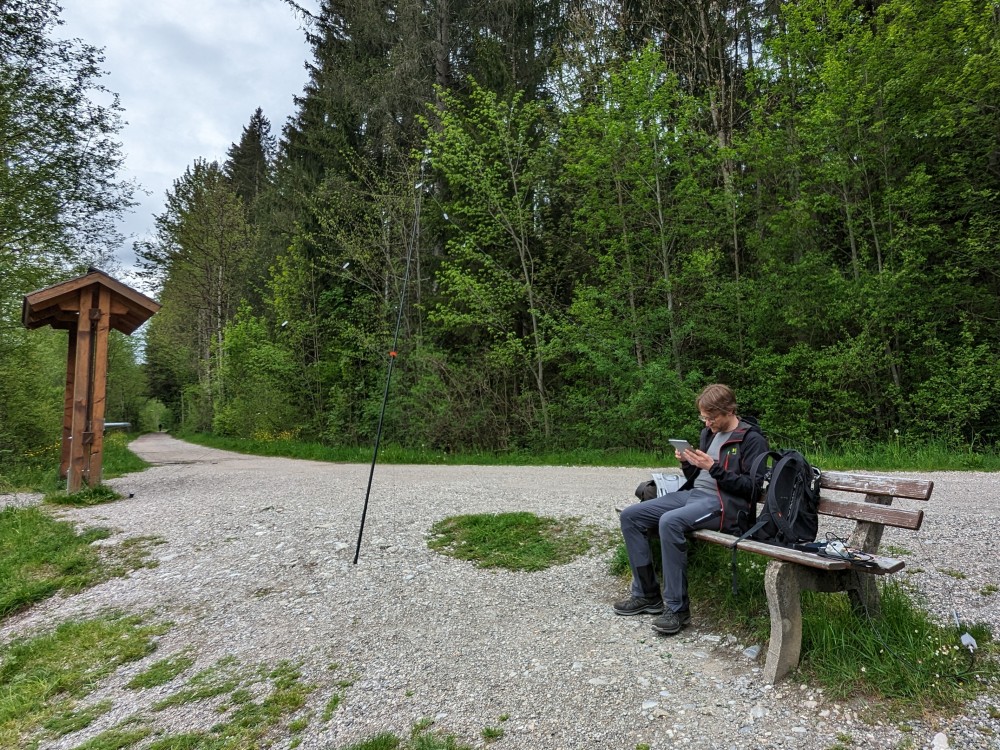
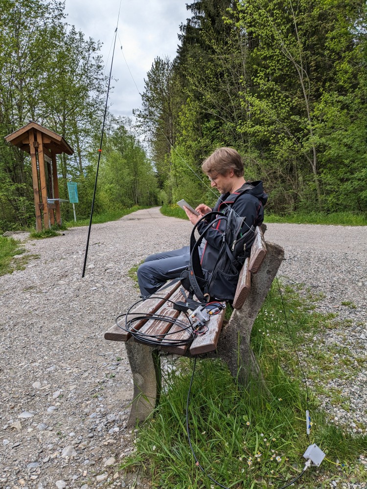
After everything was put together, I used a weekend trip to test the equipment under realistic conditions. The first test was conducted at the Illerursprung (Locator JN57dk). After calling CQ as DC6GF/P, I was a bit overwhelmed by the response and also by only being able to use the touch display. So sorry to all who received weird messages from me at that day! In the end six QSOs from a not so optimal location within a valley were a big success for me.
Tourist information board at the Illerursprung.
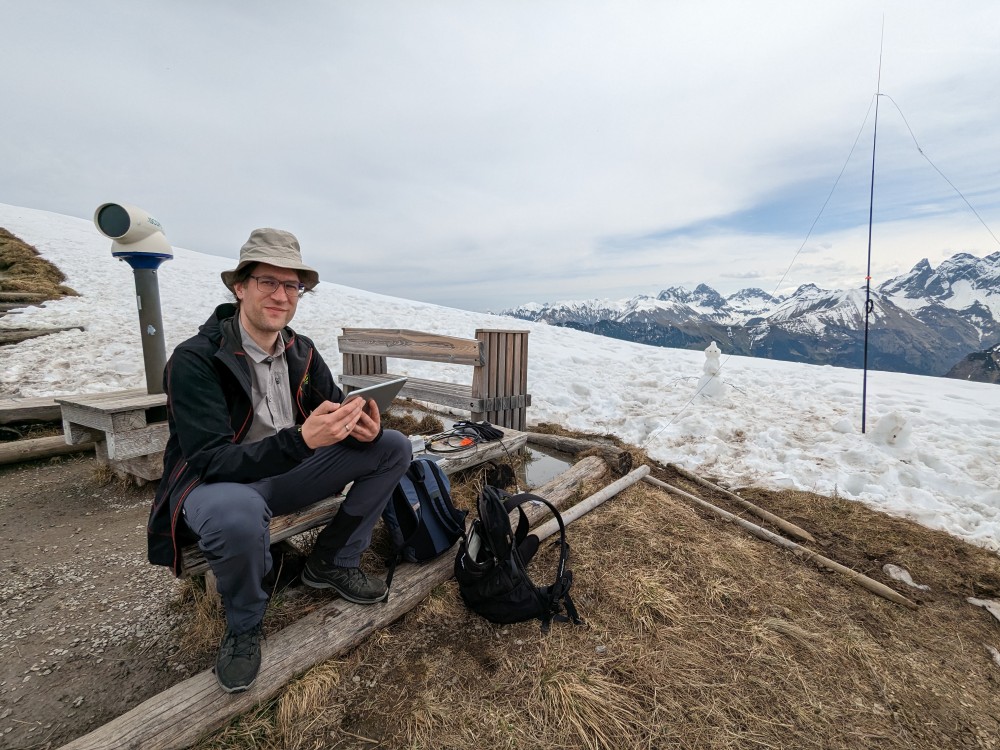
The next test was operating from nearby the Fellhorn summit (Locator JN57ci). There I struggled with difficult lighting conditions and usability issues of the VNC client together with the desktop environment that would switch to a different desktop when touching in the wrong place. Returning to the right desktop was unequally difficult. In the end I achieved only two QSOs.
DC6GF waiting for the next QSO near the Fellhorn summit.
The last test with a refined end-fed antenna was conducted directly from my garden. As everything worked well, this setup was the final one and could be packed for the trip to Iceland.
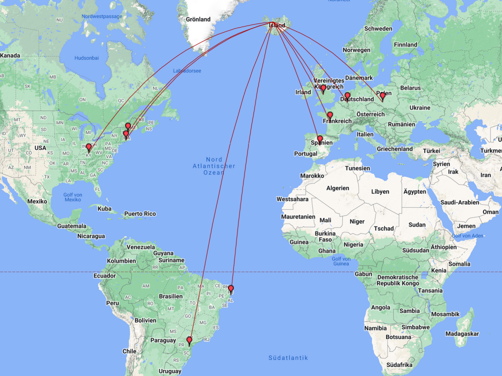
On the Air as TF/DC6GF
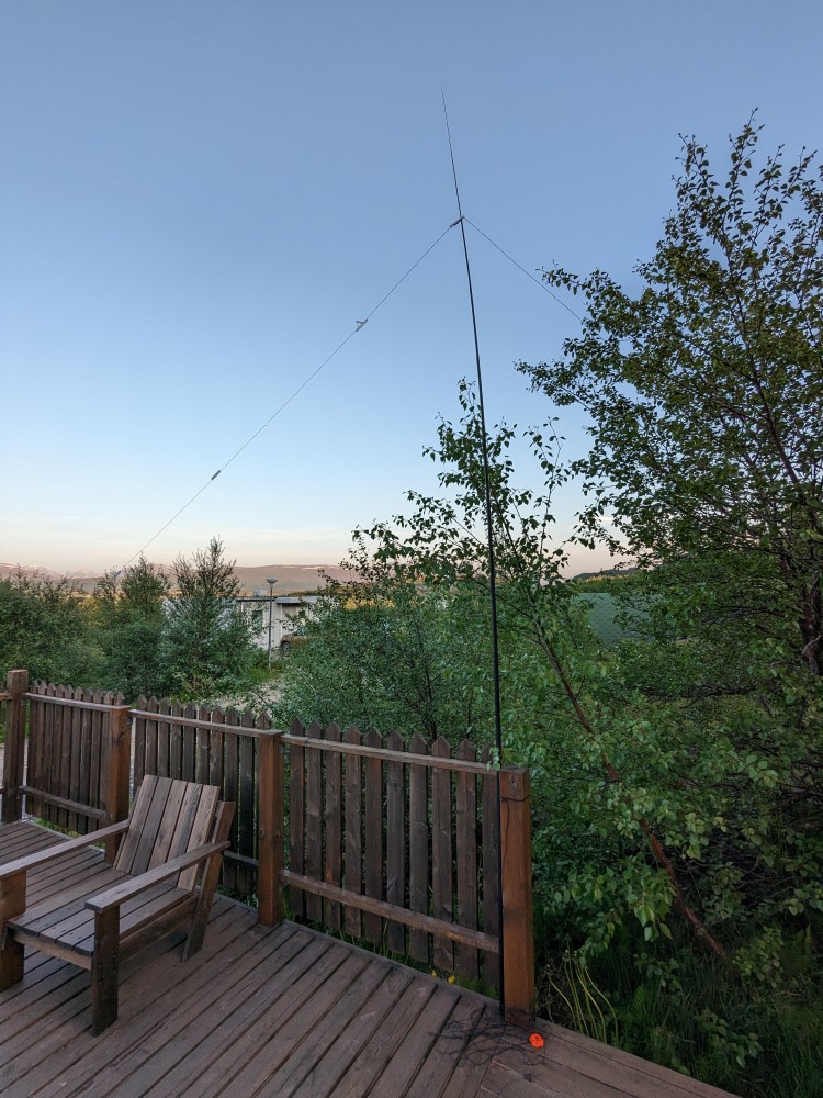
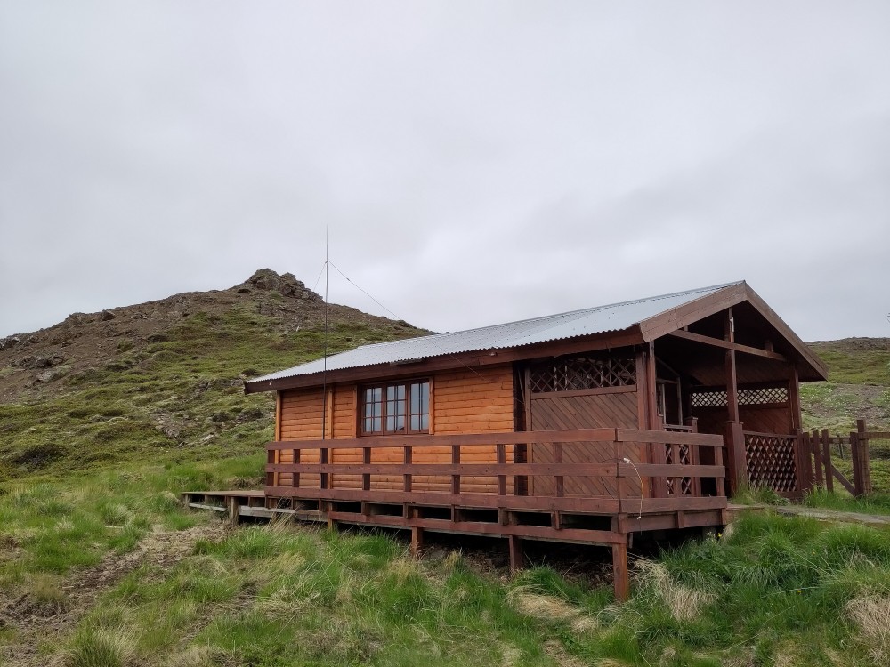
On Iceland, operation was planned from four different locations where we did not stay at a hotel but at cottages where there was some space outside to place the antenna. The locators I operated from were HP94sg (7th June 2023), IP25sg (11th and 12th June), IP05am (17th June), and HP85pa (18th and 19th June).
View from the QTH in IP25.The setup at IP05.The QTH in HP85 with the antenna mast mounted to the wooden fence of the cottage.Evening at the HP85 QTH.
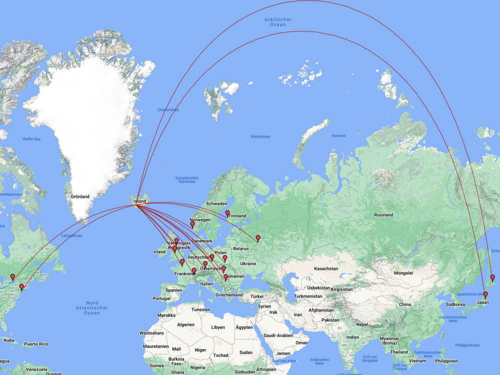
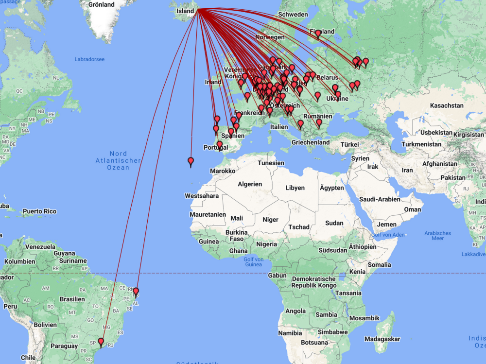
The number of QSOs varied strongly between 6 QSOs on two days from HP85, and 75 QSOs on two days from IP25. Highlights were some QSOs to Japan and Brazil. ODX was PY5EJ in GG54 with a distance of 10418km. Impressive how far 4W of RF power can go! Overall I achieved 107 QSOs (43 on 20m, 37 on 17m, and 27 on 15m) with 105 individuals from 27 DXCC entities. I put some overview graphs below. Please excuse the poor quality and German localization but I think the main information is visible.
QSOs from HP94QSOs from IP25QSOs from IP05QSOs from HP85
Conclusion
Operating from not so usual locations proved to be a lot of fun and a great experience. So whenever the occasion comes up again, I will definitely try again.
Some time ago I ordered a (tr)uSDX kit and assembled it according to the video instructions by Manuel (DL2MAN). The assembly itself went quite smooth. However, the tuning took some time and although there were no real surprises, some information for success was hidden in the depth of the discussion groups. So I thought summarizing them here might be helpful.
Tuning the Filters
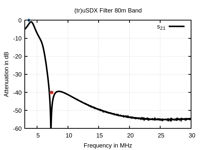
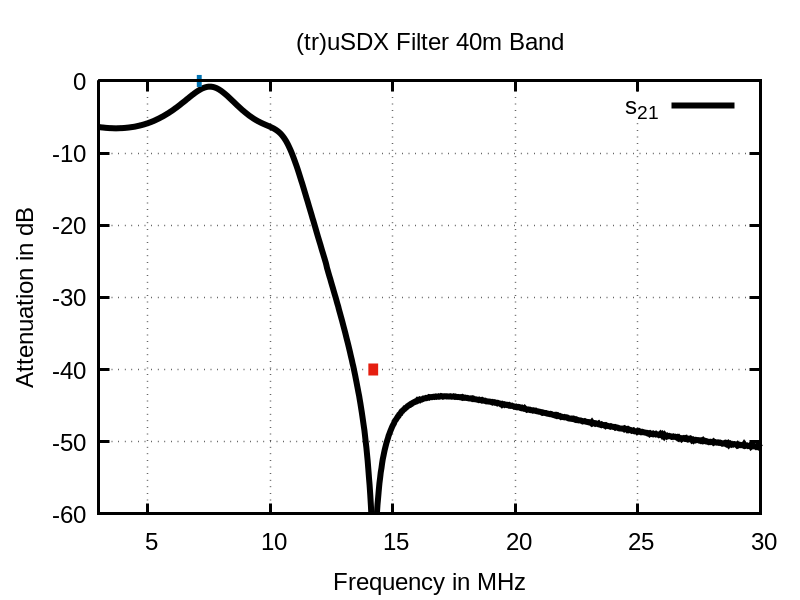
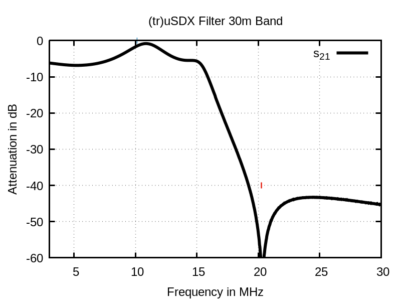
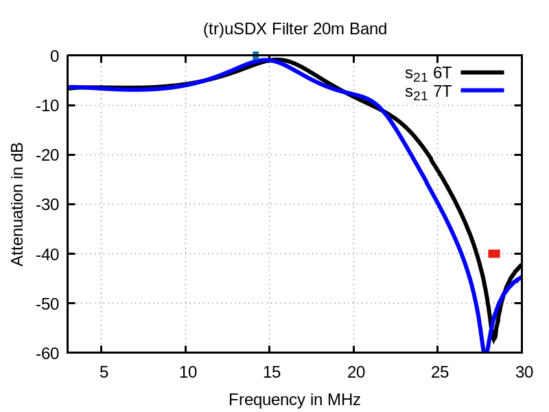
Tuning the filters is already explained quite well in the video tutorial. For reference, here are the actual filter curves I achieved after tuning. I indicated the passband with a wide blue line at 0dB and the first harmonic with a wide red line at -40dB.
For 20m, I was not able to put the notch high enough in frequency to reach the desired stop band with the number of turns given in the instructions, so I removed one turn. After that I had to struggle to move the notch down in frequency to fit the stop band. In the end I succeeded but as one can see from the graph, I could have left the coil as it was because the additional suppression is marginal.
Tuning Rshunt
After tuning the filters, I wanted to tune the efficiency of the amplifier but could not reach more than about 68%. After some digging through the forum, I found the solution in the quite low Rshunt value setting in my firmware. It was set to 17, where a setting of 19 is more reasonable for my setup. After that, I was able to tune the efficiency in the desired region above 75%.
The procedure to determine the correct value for Rshunt is quite straight forward:
Measure the receive power consumption PRx of your (tr)uSDX. I reduced the output volume to the point where the current did not decrease any more for lower volumes.
Measure the transmit power consumption PTX and the RF output power PRF.
Compute the efficiency by eff = PRF/(PTX-PRX).
Tune Rshunt to match the computed efficiencies over the different bands to the displayed values.
I took measurements over all bands and was able to match the measured and the displayed efficiency quite well but not perfectly which cannot be expected from the small device.
Tuning the Efficiency
After setting the correct Rshunt value, tuning the efficiency for the lower bandy went as described in the video tutorial. For the 20m band however, the output power was quite low and the efficiency also not very good. So I removed one turn from the coil and was also able to achieve about 4.5 to 5W of RF output power at a decent efficiency.
Using it with WSJT-X on a Raspberry Pi
In order to successfully use CAT control on Linux, you have to execute the following command to successfully access the interface:
stty -F /dev/ttyUSB0 raw -echo -echoe -echoctl -hupcl -echoke 38400
The command has to be executed before accessing the interface but it worked as well while WSJT-X was already running. Before the command, the CAT control failed, after the command, everything worked as expected.
Summary
Thanks to DL2MAN and PE1NNZ for this great device!
Important Links
The original posts from the forum, where I found the information given above:
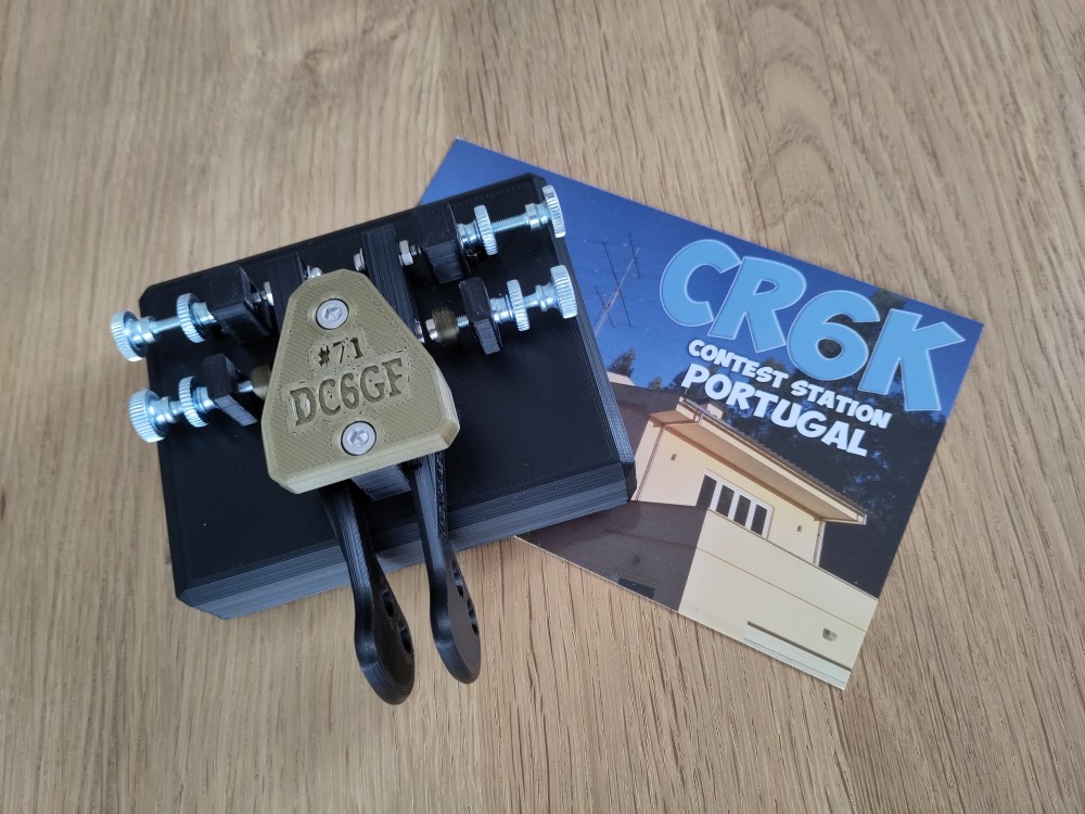
Yesterday a new tool arrived that was still missing for my radio station: A CW paddle made by Filipe, CT1ILT. Now I have no more excuse to not start practicing CW. I wonder how long I need to be ready for my first CW QSO.